
Table of Contents
Q.1. Define Marketing Research. Enumerate the critical factors in organising a good marketing research study. Substantiate your answer with suitable examples from the hospitality industry. (20)
Market research is the process of gathering, analysing and interpreting information about a market, about a product or service to be offered for sale in that market, and about the past, present and potential customers for the product or service; research into the characteristics, spending habits, location and needs of your business’s target market, the industry as a whole, and the particular competitors you face.
Accurate and thorough information is the foundation of all successful business ventures because it provides a wealth of information about prospective and existing customers, the competition, and the industry in general. It allows business owners to determine the feasibility of a business before committing substantial resources to the venture.
Market research provides relevant data to help solve marketing challenges that a business will most likely face–an integral part of the business planning process. In fact, strategies such as market segmentation (identifying specific groups within a market) and product differentiation (creating an identity for a product or service that separates it from those of the competitors) are impossible to develop without market research.
The critical factors in organising a good marketing research study
Marketing research must not be mere collection of statistical information, One must justify the choice of methodology of data collection and analysis. And, the researcher must not be too much pre-occupied with techniques, but instead convey the meaning of the results in the marketing language even when some advanced or sophisticated tool is being used. Likewise, marketing manager(s) should also provide a clear, detailed scenario of the problems faced by the company before the marketing researchers (s). They must allow adequate time and budget for conducting the study. They must not use marketing research as a fire fighting device or to justify some preconceived action(s).
Marketing research is the function that likes the consumer with the organisation through information. It involves systematic and objective search for and analysis of information that , can be used for evolving some marketing decisions.
Any research study must clearly state the issues being investigated. It must apply systematic and formal procedure in collection and analysis of information. It must communicate the study findings in a manner which could help in arriving at some marketing decisions.
A research study ‘will fail to serve its purpose if marketing researcher merely collates some statistical facts or is pre-occupied with techniques or uses data of questionable validity or communicates the findings in too much vague or technical language.
Likewise, a research study will suffer if the marketing manager does not offer full perspective of the research problem; or allows inadequate time; or uses research as a fire-fighting device or does not really appreciate the value of research.
Problem must be clearly defined and reasons for undertaking the research from the point of view of marketing decision making should be explicitly justified.
In order to carry out effective research programme
1. Prepare a list of objectives to be examined
2. Avoid
• Vague terms of reference
• Trivial research projects
• Research where underlying purpose is unknown or with held.
3. Ensure concurrence about the terms of references (specially research objectives; plan of data collection, time and budget) among all concerned.
Q.2. Define Primary and Secondary Data. Explain their role in surveys with suitable examples. What precautions would you take before using secondary data? (20)
Primary Data
These are the data which are collected from some primary sources i.e., a source of origin where the data generate.These are collected for the first time by an investigator or an agency for any statistical analysis.
“Data which are gathered originally for a certain purpose are known as primary data.” — Horace Secrist
Merits
1. It has high degree of accuracy.2. For some enquiries, secondary data is not available.
3. These are more reliable.
4. It needs no extra precautions.
Demerits
1. It requires lot of time.2. It needs much money.
3. These data can be obtained though skilled persons only.
4. Sometimes, these data are not available altogether.
Secondary data
These are the data which are collected from some secondary source i.e. the source of reservation storage where the data is collected by one person and used by other agency. These are collected as primary data and used by other as secondary data.“The data which are used in an investigation, but which have been gathered originally by someone else for some other purpose are known as secondary data.” — Blair
Merits
1. It is easy to collect.2. Time and money is saved.
3. Sometimes primary data cannot be obtained.
4. Some data are more reliable than primary.
Demerits
1. These are not reliable as primary data.2. Extra caution is needed to use these data.
3. All types of data are not available.
4. Purpose of original collection may have been different.
Role of data in surveys
Among the communication methods in use today, surveys involving structured questionnaires are the most extensively used.
E.g. – If you want to know the consumption patterns of a particular product category, reasons for brand choice, the relative influence of different media on a person’s decisions,
The natural course would be to ask the people themselves. In order to get comparable information from respondents, formal nondisguised questions are predesigned in the form of a questionnaire.
Administrating the questionnaire may involve participation of an interviewer, who is instructed to ask the questions in the order given on the form and to ask only those questions. The questionnaire method, with or without the participation of an interviewer is such a prevalent and versatile method of data collection that it was felt that various stages of questionnaire planning and execution warranted a detailed explanation.
The basic advantages of using questionnaires are versatility and economy. The questionnaire method is versatile enough to be tailored to the needs of most marketing research situations. In addition variables like knowledge, opinions, intentions, motivations and personal habits which do not lend themselves to observation, can only be elicited through questioning. It is also the only method to get information on past events for which records have not been maintained.
Relatively speaking, questioning turns out to be speedier and less costly then observation. Interviewers using questionnaires have a higher degree of control over information gathering activities than do observers, who have to wait for the respondent to perform the action under study. Moreover the lag time between one interview and another is controllable by the interviewer while the wait time between two successive observations cannot be controlled by the observer.
The survey questionnaire method is however subject to certain limitations also. Important among them are inability of the respondent to furnish information. Even though they may be willing to share information ‘about themselves, many respondents are actually unable to give accurate, information to the questions asked.
For example, it might be difficult for you, at a point of time to give the exact reason of choosing a brand of soap over another unless you have carefully analysed these reasons beforehand.
Therefore, on questions of buyer motivations quite often inaccurate information is given which interferes with the reliability of data collected.
Precautions that should be taken while using Secondary Data
The investigator should take precautions before using the secondary data. In this connection, following precautions should be taken into account.1. Suitable Purpose of Investigation
The investigator must ensure that the data are suitable for the purpose of enquiry.2. Inadequate Data
Adequacy of the data is to be judged in the light of the requirements of the survey as well as the geographical area covered by the available data.3. Definition of Units
The investigator must ensure that the definitions of units which are used by him are the same as in the earlier investigation.4. Degree of Accuracy
The investigator should keep in mind the degree accuracy maintained by each investigator.5. Time and Condition of Collection of Facts
It should be ascertained before making use of available data to which period and conditions, the data was collected.6. Comparison
Investigator should keep in mind whether the secondary data’ reasonable, consistent and comparable.7. Test Checking
The use of the secondary data must do test checking and see that totals and rates have been correctly calculated.8. Homogeneous Conditions
It is not safe to take published statistics at their face value without knowing their means, values and limitations.Q.3. Distinguish clearly between Structured and Unstructured Questionnaire. Construct a suitable questionnaire containing not more than ten questions pertaining to ‘Consumer survey on Star category hotel”. (20)
Unstructured Questionnaire
An unstructured questionnaire is an instrument or guide used by an interviewer who asks questions about a particular topic or issue. Although a question guide is provided for the interviewer to direct the interview, the specific questions and the sequence in which they are asked are not precisely determined in advance. The questions to be asked are kept flexible in their own words and also the respondents are allowed to answer the questions in a manner they like.Structured Questionnaire
A structured questionnaire, on the other hand, is one in which the questions asked are precisely decided in advance. When used as an interviewing method, the questions are asked exactly as they are written, in the same sequence, using the same style, for all interviews. Nonetheless, the structured questionnaire can sometimes be left a bit open for the interviewer to amend to suit a specific context. It is the one in which the question to be asked and responses permitted are explicitly pre-specified.Questionnaire on “Consumer survey on Star category hotel”
1. How friendly was the Hotel staff
a. Extremely Friendly
b. Quite Friendly
c. Moderate Friendly
d. Somewhat Friendly
2. How polite was the hotel staff?
a. Extremely Polite
b. Quite Polite
c. Moderate Polite
d. Somewhat Polite
3. How quick was the check-in process?
a. Extremely Quick
b. Quite Quick
c. Moderate Quick
d. Somewhat Quick
4. How clean was your room upon arrival?
a. Extremely Clean
b. Quite Clean
c. Moderate Clean
d. Somewhat Clean
5. How well equipped was your room?
a. Extremely
b. Quite
c. Moderate
d. Somewhat
6. How quickly hotel staff respond to your requests?
a. Extremely Quick
b. Quite Quick
c. Moderate Quick
d. Somewhat Quick
7. How likely you will recommend hotel to a friend?
a. Extremely likely
b. Quite likely
c. Moderate likely
d. Somewhat likely
8. How affordable were the services?
a. Extremely good
b. Quite good
c. Moderate good
d. Somewhat good
9. How affordable stay was at the hotel?
a. Extremely good
b. Quite good
c. Moderate good
d. Somewhat good
10. How likely are you to stay at hotel again?
a. Extremely likely
b. Quite likely
c. Moderate likely
d. Somewhat likely
Q.4. Answer the following questions in about 300 words each:
a. Critically examine the various probability sampling methods. (10)
Probability Sampling Methods
1. Simple Random Sampling
Under this sampling design, each member of the population has known and equal probability of being included in the sample. Simple random sampling is not widely used in marketing research because of the following reasons.• In consumer research studies, we usually select individuals, households, shops or areas as the sampling units. It may not be easy to prepare a sampling frame as it is very difficult to get lists of households, individuals and shops, although areas may be completely represented through maps.
• We know that an industry comprises of various firms of different sizes. If one wants to study some aspects of an industry, one might like to choose a sampling design where there is a higher probability of a larger firm being selected. If that is the case, the very concept of simple random sampling becomes inapplicable in such situations. The simple random sampling has some applications in Industrial Marketing where generally purchasing agents or companies or areas are the sampling units which are usually not very big in number. Therefore, it becomes easy to prepare a sampling frame thus facilitating the use of simple random sampling.
2. Systematic Sampling
The mechanics of taking a systematic sample are very simple. Systematic sampling is a case of mixed sampling where both probabilistic and non-probabilistic methods of choosing a sample are used. This is because the first unit of the sample is selected at random between numbers 1 and K (probabilistic method) and then the rests of the units of the sample are fixed by the choice of the first member (non-probabilistic method).It is very likely that systematic sampling would result into more representative sample than simple random sampling. In systematic sampling the elements of the population are ordered in a particular fashion.
Example – we want to estimate the sales of all the retail stores in Delhi. Under a simple random sampling, if we draw a random sample of size n, it is very likely that Most of the sampled stores might turn out to be low sales volume store. However, in systematic sampling we order these retail stores according to ascending or descending order of sales, therefore, a systematic sample would definitely contain some low volume and high volume retail stores. Thus, a systematic sample is likely to be more representative than a sample random sample. A systematic sample might also reduce the representativeness of the sample.
3. Stratified random sampling
It involves a method where the researcher divides a more extensive population into smaller groups that usually don’t overlap but represent the entire population. While sampling, organize these groups and then draw a sample from each group separately.A standard method is to arrange or classify by sex, age, ethnicity, and similar ways. Splitting subjects into mutually exclusive groups and then using simple random sampling to choose members from groups.
Members of these groups should be distinct so that every member of all groups get equal opportunity to be selected using simple probability. This sampling method is also called “random quota sampling.”
In stratified sampling, the entire population is divided into various mutually exclusive and collectively exhaustive strata (groups). By mutually, exclusive it is meant that if an element of a group belongs to one strata, then it doesn’t belong to any other strata.
4. Cluster Sampling
If we divide all the elements of the population into suitable, clusters; and select few clusters randomly and all the elements of the selected clusters are used, then this method of sampling is called cluster sampling’.This method of collecting data is cheaper since collection of data fear nearby units is easier, faster and more convenient than collecting data over units scattered over a region. For instance, it would not only be cheaper but also convenient to collect data on all households in a sample of few villages.(clusters) than to surrey a sample of the same number of households selected randomly from a list of all households.
The criteria for dividing the population into mutually exclusive and collectively exhaustive clusters is, that the elements in the clusters should be as heterogeneous as possible and elements between cluster should be as homogeneous as possible.
5. Area Sampling
In a marketing research study involving sampling of population which may be grouped according to geographical areas (blocks), Census tracts, Communities, constituencies etc., another version of cluster sampling namely Area Sampling is used.The entire area is divided into various clusters. The cluster may or may not be of equal size. Below we will discuss a sampling scheme where sampling is done by taking into account the size of the cluster. This type of design is called probability proportional to size sampling.
b. What do you understand by ‘Sample Design” ? What points should be taken into consideration in developing sample survey design? (10)
Sample Design
A sample design is the framework, or road map, that serves as the basis for the selection of a survey sample and affects many other important aspects of a survey as well. In a broad context, survey researchers are interested in obtaining some type of information through a survey for some population, or universe, of interest. One must define a sampling frame that represents the population of interest, from which a sample is to be drawn. The sampling frame may be identical to the population, or it may be only part of it and is therefore subject to some undercoverage, or it may have an indirect relationship to the population (e. g. the population is preschool children and the frame is a listing of preschools).The sample design describes the procedure by which sample is selected. There is two classes of methods by which samples can be selected. They are probability & non- probability.
Points that should be taken into consideration in developing sample survey design
While developing a sampling design, the researcher must pay attention to the following points:
1. Type of universe
The first step in developing any sample design is to clearly define the set of objects, technically called the Universe, to be studied. The universe can be finite or infinite. In finite universe the number of items is certain, but in case of an infinite universe the number of items is infinite, i.e., we cannot have any idea about the total number of items. The population of a city, the number of workers in a factory and the like are examples of finite universes, whereas the number of stars in the sky, listeners of a specific radio programme, throwing of a dice etc. are examples of infinite universes.2. Sampling unit
A decision has to be taken concerning a sampling unit before selecting sample. Sampling unit may be a geographical one such as state, district, village, etc., or a construction unit such as house, flat, etc., or it may be a social unit such as family, club, school, etc., or it may be an individual. The researcher will have to decide one or more of such units that he has to select for his study.3. Source list
It is also known as ‘sampling frame’ from which sample is to be drawn. It contains the names of all items of a universe (in case of finite universe only). If source list is not available, researcher has to prepare it. Such a list should be comprehensive, correct, reliable and appropriate. It is extremely important for the source list to be as representative of the population as possible.4. Size of sample
This refers to the number of items to be selected from the universe to constitute a sample. This a major problem before a researcher. The size of sample should neither be excessively large, nor too small. It should be optimum. An optimum sample is one which fulfills the requirements of efficiency, representativeness, reliability and flexibility. While deciding the size of sample, researcher must determine the desired precision as also an acceptable confidence level for the estimate. The size of population variance needs to be considered as in case of larger variance usually a bigger sample is needed. The size of population must be kept in view for this also limits the sample size.5. Parameters of interest
In determining the sample design, one must consider the question of the specific population parameters which are of interest. For instance, we may be interested in estimating the proportion of persons with some characteristic in the population, or we may be interested in knowing some average or the other measure concerning the population. There may also be important sub-groups in the population about whom we would like to make estimates. All this has a strong impact upon the sample design we would accept.6. Budgetary constraint
Cost considerations, from practical point of view, have a major impact upon decisions relating to not only the size of the sample but also to the type of sample. This fact can even lead to the use of a non-probability sample.7. Sampling procedure
Finally, the researcher must decide the type of sample he will use i.e., he must decide about the technique to be used in selecting the items for the sample. In fact, this technique or procedure stands for the sample design itself. There are several sample designs (explained in the pages that follow) out of which the researcher must choose one for his study. Obviously, he must select that design which, for a given sample size and for a given cost, has a smaller sampling error.Q.5. What are the four different levels of measurement ? Discuss the mathematical operations which may or may not be used under each level of measurement. (20)
Nominal Scale
A Nominal Scale is a measurement scale, in which numbers serve as “tags” or “labels” only, to identify or classify an object. A nominal scale measurement normally deals only with non-numeric (quantitative) variables or where numbers have no value.Below is an example of Nominal level of measurement.
Please select the degree of discomfort of the disease:
1-Mild
2-Moderate
3-Severe
In this particular example, 1=Mild, 2=Moderate, and 3=Severe. Here numbers are simply used as tags and have no value.
There are four variable measurement scales: nominal, ordinal, interval and ratio. These measurement scales are ways to categorize different variables (an element, feature or factor that is likely to vary). By default, all variables fall in one of the four scales mentioned above. Understanding their properties and assigning variables to one of the four measurement scales is important mathematically because they determine what mathematical operations are allowed.
Nominal scale possesses only the description characteristic which means it possesses unique labels to identify or delegate values to the items. When nominal scale is used for the purpose of identification, there is a strict one-to-one correlation between an object and the numeric value assigned to it. For example, numbers are written on cars in a racing track. The numbers are there merely to identify the driver associated with the car, it has nothing to do with characteristics of the car.
But when nominal scale is used for the purpose of classification, then the numbers assigned to the object serve as tags to categorize or arrange objects in class. For example, in the case of a gender scale, an individual can be categorized either as male or female. In this case, all objects in the category will have the same number, for example, all males can be no. 1 and all females can be no. 2. Please note, that nominal is purely used for counting purposes.
For example, let’s assume we have 5 colours, orange, blue, red, black and yellow. We could number them in any order we like either 1 to 5 or 5 to 1 in ascending or descending order. Here numbers are assigned to colours only to identify them. Another example of nominal scale from a research activity point to view is YES/NO scale. It essentially has no order.
Characteristics of Nominal Scale
• In nominal scale a variable is divided into two or more categories, for example, agree/disagree, yes or no etc. It’s is a measurement mechanism in which answer to a particular question can fall into either category.
• Nominal scale is qualitative in nature, which means numbers are used here only to categorize or identify objects. For example, football fans will be really excited, as the football world cup is around the corner! Have you noticed numbers on a jersey of a football player? These numbers have nothing to do with the ability of players, however, they can help identify the player.
• In nominal scale, numbers don’t define the characteristics related to the object, which means each number is assigned to one object. The only permissible aspect related to numbers in a nominal scale is “counting.”
b. Ordinal Scale
Ordinal scale is the 2nd level of measurement that reports the ranking and ordering of the data without actually establishing the degree of variation between them. Ordinal level of measurement is the second of the four measurement scales.“Ordinal” indicates “order”. Ordinal data is quantitative data which have naturally occurring orders and the difference between is unknown. It can be named, grouped and also ranked.
For example:
“How satisfied are you with our products?”
1- Totally Satisfied
2- Satisfied
3- Neutral
4- Dissatisfied
5- Totally Dissatisfied
Survey respondents will choose between these options of satisfaction but the answer to “how much?” will remain unanswered. The understanding of various scales helps statisticians and researchers so that the use of data analysis techniques can be applied accordingly.
Thus, an ordinal scale is used as a comparison parameter to understand whether the variables are greater or lesser than one another using sorting. The central tendency of the ordinal scale is Median.
Likert Scale is an example of why the interval difference between ordinal variables cannot be concluded. In this scale the answer options usually polar such as, “Totally satisfied” to “Totally dissatisfied”.
The intensity of difference between these options can’t be related to specific values as the difference value between totally satisfied and totally dissatisfied will be much larger than the difference between satisfied and neutral. If someone loves Mercedes Benz cars and is asked “How likely are you to recommend Mercedes Benz to your friends and family?” will be troubled to choose between Extremely likely and Likely. Thus, an ordinal scale is used when the order of options is to be deduced and not when the interval difference is also to be established.
Ordinal Scale Characteristics
• Along with identifying and describing the magnitude, the ordinal scale shows the relative rank of variables.• The properties of the interval are not known.
• Measurement of non-numeric attributes such as frequency, satisfaction, happiness etc.
• In addition to the information provided by nominal scale, ordinal scale identifies the rank of variables.
• Using this scale, survey makers can analyse the degree of agreement among respondents with respect to the identified order of the variables.
c. Interval Scale
The interval scale is a quantitative measurement scale where there is order, the difference between the two variables is meaningful and equal, and the presence of zero is arbitrary. It measures variables that exist along a common scale at equal intervals. The measures used to calculate the distance between the variables are highly reliable.The interval scale is the third level of measurement after the nominal scale and the ordinal scale. Understanding the first two levels will help you differentiate interval measurements. A nominal scale is used when variables do not have a natural order or ranking. You can include numbered or unnumbered variables, but common survey examples include gender, location, political party, pets, and so on.
In contrast, on an ordinal scale, the rank of variables matters, but the difference or distance between the variables doesn’t. Think about price range filters for online shopping. You can select “less than $25,” “$26 up to $50,” and so forth, but the difference between them is not relevant. Likewise, the ranking of variables such as “Would not recommend” and “Would highly recommend” matters, but the difference between them does not unless that difference is represented by another variable.
The general mathematical form of interval scale is given by the equation.
Y = a+ bX
Characteristics of interval scale
• The interval scale is preferred to nominal scale or ordinal scale because the latter two are qualitative scales. The interval scale is quantitative in the sense that it can quantify the difference between values.
• Interval data can be discrete with whole numbers like 8 degrees, 4 years, 2 months, etc., or continuous with fractional numbers like 12.2 degrees, 3.5 weeks or 4.2 miles.
• You can subtract values between two variables that help understand the difference between two variables.
• Interval measurement allows you to calculate the mean and median of variables.
• Interval data is especially useful in business, social, and scientific analysis and strategy because it is straightforward and quantitative.
• This is a preferred scale in statistics because you can assign a numerical value to any arbitrary assessment, such as feelings and sentiments.
d. Ratio Scale
Ratio scale is a type of variable measurement scale which is quantitative in nature. Ratio scale allows any researcher to compare the intervals or differences. Ratio scale is the 4th level of measurement and possesses a zero point or character of origin. This is a unique feature of ratio scale. For example, the temperature outside is 0-degree Celsius. 0 degree doesn’t mean it’s not hot or cold, it is a value.The mathematical form of the measurement is written as
Y=bX
Following example of ratio level of measurement to help understand the scale better.
Please select which age bracket do you fall in?
• Below 20 years
• 21-30 years
• 31-40 years
• 41-50 years
• 50 years and above
Ratio scale has most of the characteristics of the other three variable measurement scale i.e. nominal, ordinal and interval. Nominal variables are used to “name,” or label a series of values. Ordinal scales provide a sufficiently good amount of information about the order of choices, such as one would be able to understand from using a customer satisfaction survey. Interval scales give us the order of values and also about the ability to quantify the difference between each one. Ratio scale helps to understand the ultimate-order, interval, values, and the true zero characteristic is an essential factor in calculating ratios.
A ratio scale is the most informative scale as it tends to tell about the order and number of the object between the values of the scale. The most common examples of ratio scale are height, money, age, weight etc. With respect to market research, the common examples that are observed are sales, price, number of customers, market share etc.
Characteristics of Ratio Scale
• Ratio scale, as mentioned earlier has an absolute zero characteristic. It has orders and equally distanced value between units. The zero point characteristic makes it relevant or meaningful to say, “one object has twice the length of the other” or “is twice as long.”
• Ratio scale doesn’t have a negative number, unlike interval scale because of the absolute zero or zero point characteristic. To measure any object on a ratio scale, researchers must first see if the object meets all the criteria for interval scale plus has an absolute zero characteristic.
• Ratio scale provides unique possibilities for statistical analysis. In ratio scale, variables can be systematically added, subtracted, multiplied and divided (ratio). All statistical analysis including mean, mode, the median can be calculated using ratio scale. Also, chi-square can be calculated on ratio scale variable.
Q.6. What are the general rules of framing a frequency distribution with particular reference to the choice of class-interval and number of classes ? Illustrate with examples. (20)
Rules of framing a frequency distribution
Tabular organization of data showing the distribution of data in classes or groups, along with the number of observations in each class or group, is called a frequency distribution. The class frequency refers to the number of observations in a particular class. Frequency distributions is a powerful statistical tools which frequently used for descriptive and predictive analytics.
The following are some five fundamental roles that should be kept in mind when constructing a grouped frequency distribution.
1. Number of class
The number of classes pretty much depends on the size of the data. In statistics, it is a common practice to keep the number of classes between 5 and 20. Too many classes will kill the purpose of data condensation into meaningful groups. At the same time, too few classes will result in a loss of information. Therefore, we always need to strike an appropriate balance.2. Range of variables
It is vital to determine the range of variable data by taking the difference between the largest and the smallest values in the data. The range of a variable allows us to pick up the correct number of classes.3. Class interval- divide range by number of class
To determine the approximate width or class interval, divide range (from step 2) by the number of classes and round to next higher whole number. The result of the division will give us equal class-interval. If equal class-intervals are inconvenient or maybe undesirable, then classes of unequal size are used. But in practice, intervals that are multiples of 5 or 10, are commonly used as people can understand them easily.4. Determine class limits
The lowest class usually starts with the smallest data value or a number less than it. It is better if it is a multiple of class-interval. Find the upper-class boundary by adding the width of the class-interval to the lower class-boundary and write down the upper-class limits too. The open-end classes, i.e., classes with the lowermost or uppermost class boundary unknown, should be avoided if possible.By adding the class-interval repeatedly, you should determine the remaining class-limits and class boundaries. We should place the lowest class at the top, and the rest should follow according to size. In some cases, we may prefer to put the highest class at the top.
5. Distribute data into classes
The best way to distribute the data into the appropriate classes is by using a “Tally-Column” where values are tabulated against suitable classes by merely making short bars or tally marks to represent them. It is customary for convenience in counting to place the first four bars vertically and the fifth one diagonally and to leave a space. Then we write the number of tallies in the frequency column. We usually omit the tally column in the final presentation of the frequency distribution. But in case of a small number of values, the actual values should be shown against each class to mitigate the chances of error.Finally, we need to total the frequency column to validate that all the data.
We apply these rules to raw group data, which are assumed to be continuous. In the case of discrete data that carry only integral values, the concept of a class boundary is unrealistic as there can be no points where the adjoining classes meet. Despite this logical difficulty, when the discrete data are sufficiently large, they are treated for convenience of calculations as continuous. They hence are grouped in the same way as the continuous data.
The steps in grouping may be summarized as follows:
1. Decide on the number of classes.
2. Determine the range, i.e., the difference between the highest and lowest observations in the data.
3. Divide range by the number of classes to estimate approximate size of the interval (h).
4. Find the lower class limit of the lowest class and add to it the class- interval to get the upper class limit.
5. Obtain class-limits for the remaining classes by adding the class-interval to the limits of the previous class.
6. Count numbers of frequencies in each class and check against the total number of observations.
Three methods of describing the limits of the class intervals in a frequency distribution:
Three ways of expressing the limits of the class intervals in a frequency distribution are namely exclusive method, inclusive method and true class limits.
Eg. Scores of ten students are
145, 142, 167, 189, 167, 156, 167, 153, 166,170,197
Step 1
Determine the range or gap between the highest and the lowest scores.
The highest score is 197 and the lowest is 142, so that the range is 55 (i.e. 197-142).
Step 2
Then we have to decide about the number of classes. We usually have 6 to 20 classes of equal length. If the number of scores/events is quite large, we usually have 10 to 20 classes. The number of classes when less than 10 is considered only when the number of scores/values is not too large.
Accordingly, an interval of 5 is chosen as best suitable to the data.
Step 3
The formula can also be used to decide about length of class interval or h, if we know the range of scores and number of classes used in grouping, as
Length of class interval- R/no. Of class
Step 4
Having determined the length of class interval and No. of classes, one must decide where to start the classes. The lowest score is 142, so we might begin with 140 as it is common to let the first class start with a number which is multiple of class interval (h).
Step 5
After writing the 12 class intervals in ascending order from bottom to top and putting tallies against the concerned class interval for each of the scores, we present the frequency distribution.
Step 6
Tally the scores in their proper intervals as shown in Table 2.6. In the first column of the table the class intervals have been listed serially from the smallest scores at the bottom of the column to the largest scores at the top. Each class interval covers 5 scores. The first interval “140 up to 145” begins with score 140 and ends with 144, thus including the 5 scores 140, 141, 142, 143 and 144.
The second class interval “145 up to 150” begins with 145 and ends with 149. The topmost class interval “195 to 200′ begins with score 195 and ends with 199 at the score 200, thus including 195, 196, 197, 198 and 199.
Let us take the first score in the first column i.e. 185. The score 185 is in the class interval “185-190” but not in “180-185”, so a tally (/) is marked against “185-190”. The second score in the first column is 147, which lies in the class interval “145-150”, so a tally (/) is marked against “145-150”. Similarly, by taking, all the 50 scores, tallies are put one by one. While marking the tallies, put cross mark or circle on the scores marked, as a mistake can reduce the whole process to naught.
The total tallies should be 50 i.e. total number of scores. When against a particular class interval there are four tallies (////) and you have to mark the fifth tally, cross the four tallies (////) to make it 5. So while marking the tallies we make the cluster of 5 tallies. By counting the number of tallies, the frequencies are recorded against each of class intervals. It completes the construction of table. The sum of the ‘f column is called N.
Q.7. (a) Give a brief note of the measure of central tendency together with their merits and demerits. Which is the best measure of central tendency and why? (10)
In statistics, a central tendency (or measure of central tendency) is a central or typical value for a probability distribution. It may also be called a center or location of the distribution. Colloquially, measures of central tendency are often called averages. The term central tendency dates from the late 1920s.
The most common measures of central tendency are the arithmetic mean, the median, and the mode. A middle tendency can be calculated for either a finite set of values or for a theoretical distribution, such as the normal distribution. Occasionally authors use central tendency to denote “the tendency of quantitative data to cluster around some central value.”
The central tendency of a distribution is typically contrasted with its dispersion or variability; dispersion and central tendency are the often characterized properties of distributions. Analysis may judge whether data has a strong or a weak central tendency based on its dispersion.
Mean
The arithmetic mean, or simply the mean or the average, is the sum of a collection of numbers divided by the count of numbers in the collection. The collection is often a set of results of an experiment or an observational study, or frequently a set of results from a survey.Advantages
• One makes use of all the available data so it is the most powerful measure to use.• It is good for ordinal or interval sets of data.
Disadvantage
• Sometimes the end figure is a decimal figure, which makes the data less meaningful. If there are extreme values (e.g. if a sequence was something like 3 6 4 3 40 3 then 40 is seen as extreme) it can also generate an unrepresentative figure.Mode
The mode of a set of data values is the value that appears most often. If X is a discrete random variable, the mode is the value x at which the probability mass function takes its maximum value. In other words, it is the value that is most likely to be sampled.Advantages
• The figure produced will be one that is actually in the set of numbers which is not always true for other measures of central tendency e.g. in a sequence of 3 6 3 11 4 3, the mode = 3. This number we can see is present in the sequence. However, other measures such as the mean would give us a figure of 5 (total of all number which is 30 divided by how many numbers there are which is 6) which is not part of the sequence.• It is the only measure of central tendency which is useful for nominal data.
Disadvantage
• There may be more than one modal value (known as bimodal) which makes the data less reliable.Median
The median is the middle number in a sorted, ascending or descending, list of numbers and can be more descriptive of that data set than the average. The median is sometimes used as opposed to the mean when there are outliers in the sequence that might skew the average of the values.Advantage
• Good to use with ordinal data.• It is generally unaffected by anomalies and so safer to use with extreme values.
Disadvantage
• Does not work well with small sets of data.There is no best measure of Central Tendency. It all depends on the purpose of our study/analysis, and also sometimes on the nature of the distribution of the data that we are working with. For example, if our distribution is skewed and we are looking for a central measure, mean would be an inappropriate option because it is affected by the presence of extreme observations. There Median would be more suitable, or let us say we want to see which size of shoes should a shopkeeper keep more in stock compared to the rest of the sizes, in that case Mode would be a more appropriate choice instead of mean or median. The reason why we have so many measures is because no one measure best fits all situations. Though, mean is highly used as a measure of central tendency in many cases.
(b) Under what circumstances would it be appropriate to use arithmetic mean, median and mode? Discuss. (10)
The mean, median and mode are measures of central tendency within a distribution of numerical values. The mean is more commonly known as the average. The median is the mid-point in a distribution of values among cases, with an equal number of cases above and below the median. The mode is the value that occurs most often in the distribution.
Mean
The mean (or average) is the most popular and well known measure of central tendency. It can be used with both discrete and continuous data, although its use is most often with continuous data (see our Types of Variable guide for data types). The mean is equal to the sum of all the values in the data set divided by the number of values in the data set.The mean is calculated by adding the value of each individual item in a group and dividing it by the total number of items in the group. For example, if you are at meeting of 10 people, and the sum of the ages of all attendees is 420, the mean age of the attendees is 420 divided by 10, or 42. The mean is used mostly as a general indicator for data, and works best when there are not a lot of outliers. For example, there is no way of knowing in this example whether some of the members are 90 and some are 5, or if all members are in their 40s.
Median
The median is the middle score for a set of data that has been arranged in order of magnitude. The median is less affected by outliers and skewed data.The median is the value that is the mid-point of a group of values, having an equal number of items in the group above and below it. For instance, in a room with five people aged 23, 25, 37, 44 and 87, the median age is 37, as there are an equal number of persons older and younger than 37. The median is used where strong outliers may skew the representation of the group, such as with incomes. If you have one person who earns $1 billion a year and nine other people who earn under $100,000 a year, the mean income for people in the group would be around $100 million, a gross distortion. The median income would be under $100,000, more closely representing the situation of the majority of the group.
Mode
The mode is the most frequent score in our data set. On a histogram it represents the highest bar in a bar chart or histogram. You can, therefore, sometimes consider the mode as being the most popular option.The mode is not often used in describing data, but it can be useful in certain circumstances. Here’s an example of determining a mode: If, in a room of 50 students, 30 are 7 years old and the rest are 6 or 8 years old, the mode of the ages is 7.
Use all Three
Mean, median and mode reveal different aspects of your data. Any one will give you a general idea, but may mislead you; having all three will give you a more complete picture. For example, for the data: 5, 7, 6, 127, you get a mean of 36.25 – an number that fits the arithmetic but seems a little out of place. The median, 6.5, may have more relevance to the series, but says nothing about the outlier. Since the series has no repeated numbers, it has no mode; this also reveals valuable information about your data.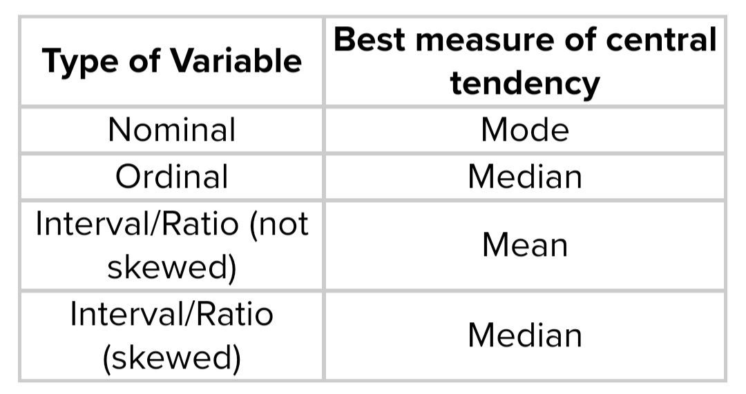
Type of Variable with Best measure of central tendency
Q.8. What is X2 (chi-square test) of goodness of fit ? What precautions are necessary while using this test ? Discuss the uses and limitations of chi-square test. (20)
A chi-squared test, also written as χ2 test, is a statistical hypothesis test that is valid to perform when the test statistic is chi-squared distributed under the null hypothesis, specifically Pearson’s chi-squared test and variants thereof. Pearson’s chi-squared test is used to determine whether there is a statistically significant difference between the expected frequencies and the observed frequencies in one or more categories of a contingency table.
Chi-Square goodness of fit test is a non-parametric test that is used to find out how the observed value of a given phenomena is significantly different from the expected value. In Chi-Square goodness of fit test, the term goodness of fit is used to compare the observed sample distribution with the expected probability distribution. Chi-Square goodness of fit test determines how well theoretical distribution (such as normal, binomial, or Poisson) fits the empirical distribution. In Chi-Square goodness of fit test, sample data is divided into intervals. Then the numbers of points that fall into the interval are compared, with the expected numbers of points in each interval.
Procedure for Chi-Square Goodness of Fit Test
Set up the hypothesis for Chi-Square goodness of fit test:
A. Null hypothesis: In Chi-Square goodness of fit test, the null hypothesis assumes that there is no significant difference between the observed and the expected value.
B. Alternative hypothesis: In Chi-Square goodness of fit test, the alternative hypothesis assumes that there is a significant difference between the observed and the expected value.
Compute the value of Chi-Square goodness of fit test using the following formula:
X² = (O-E²)/E
Where, = Chi-Square goodness of fit test O= observed value E= expected value.
Precautions about using Chi – square test
In order to use a chi-square test properly, one has to be extremely careful and keep in mind certain precautions:
1. A sample size should be large enough. If the expected frequencies are too small, the value of chi-square gets over estimated. To overcome this problem we must ensure that the observed frequency in any cell of the contingency table should not be less than 5.
2. When the calculated value of chi-square turns out to be more than the critical or theoretical value at a predetermined level of significance. We reject the null hypothesis. In contrast, when the chi-square value is less than the critical theoretical value, the null hypothesis is not rejected.
However, when the chi-square value turns out to be zero, we have to be extremely careful to confirm that there is no difference, between the observed and expected frequencies. Such a situation sometimes arises on account of faulty method used in the collection of data.
Uses of chi square test
In cryptanalysis, the chi-squared test is used to compare the distribution of plaintext and (possibly) decrypted ciphertext. The lowest value of the test means that the decryption was successful with high probability. This method can be generalized for solving modern cryptographic problems.
In bioinformatics, chi-squared test is used to compare the distribution of certain properties of genes (e.g., genomic content, mutation rate, interaction network clustering, etc.) belonging to different categories (e.g., disease genes, essential genes, genes on a certain chromosome etc.).
Limitations of Chi square test
First, chi-square is highly sensitive to sample size. As sample size increases, absolute differences become a smaller and smaller proportion of the expected value. What this means is that a reasonably strong association may not come up as significant if the sample size is small, and conversely, in large samples, we may find statistical significance when the findings are small and uninteresting., i.e., the findings are not substantively significant, although they are statistically significant.
Chi-square is also sensitive to small frequencies in the cells of tables. Generally when the expected frequency in a cell of a table is less than 5, chi-square can lead to erroneous conclusions. The rule of thumb here is that if either (i) an expected value in a cell is less than 5 or (ii) more than 20% of the expected values in cells are less than 5, then chi-square should not and usually is not computed.
Q.9. What do you understand by association of attributes ? How will you examine the consistency of data classified according to different attributes? (20)
Association of Attributes
Association of Attributes is When data is collected on the basis of some attribute or attributes, we have statistics commonly termed as statistics of attributes. It is not necessary that the objects may process only one attribute; rather it would be found that the objects possess more than one attribute. In such a situation our interest may remain in knowing whether the attributes are associated with each other or not. For example, among a group of people we may find that some of them are inoculated against small-pox and among the inoculated we may observe that some of them suffered from small-pox after inoculation.An attribute refers to the quality of a characteristic. The theory of attributes deals with qualitative types of characteristics that are calculated by using quantitative measurements. Therefore, the attribute needs slightly different kinds of statistical treatments, which the variables do not get. Attributes refer to the characteristics of the item under study, like the habit of smoking, or drinking. So ‘smoking’ and ‘drinking’ both refer to the example of an attribute.
In the theory of attributes, the researcher puts more emphasis on quality (rather than on quantity). Since the statistical techniques deal with quantitative measurements, qualitative data is converted into quantitative data in the theory of attributes.
There are certain representations that are made in the theory of attributes. The population in the theory of attributes is divided into two classes, namely the negative class and the positive class. The positive class signifies that the attribute is present in that particular item under study, and this class in the theory of attributes is represented as A, B, C, etc. The negative class signifies that the attribute is not present in that particular item under study, and this class in the theory of attributes is represented as α, β, etc.
The assembling of the two attributes, i.e. by combining the letters under consideration (such as AB), denotes the assembling of the two attributes.
This assembling of the two attributes is termed dichotomous classification. The number of the observations that have been allocated in the attributes is known as the class frequencies. These class frequencies are symbolically denoted by bracketing the attribute terminologies. (B), for example, stands for the class frequency of the attribute B. The frequencies of the class also have some levels in the attribute.
Determination of Consistency of Data
It is a well known fact that no frequency can be negative. If the frequencies of various classes are counted and any class frequency obtained comes out to be negative, then the data is said to be inconsistent. Such inconsistency arises due to wrong counting, or inaccurate addition or subtraction or sometimes due to error in printing. In order to test whether the data is consistent, all the class frequencies are calculated and if none of them is found to be negative, the data is consistent. It should be noted that if the data is consistent it does not mean that the counting is correct or calculations are accurate. But if the data is inconsistent, it means that there is either mistake or misprint in figures.In order to test the consistency of data, obtain the ultimate class frequencies. If any of them is negative, the data is inconsistent. It would also be seen that no higher order class could have a greater frequency than the lower order class frequency. If any frequency of an attribute or combination of attributes is greater than the total frequency N (frequency of zero order), the data is inconsistent. The easy way to check whether the ultimate class frequencies are negative or not (i.e. checking the data for consistency), is to enter the class frequencies. This will present an overall picture of all the ultimate class frequencies. It is also possible to lay down conditions for consistency of data.
Q.10. What is regression ? Why are there, in general, two regression lines ? Under what conditions can There be only one regression line? (20)
Regression
Regression is a statistical method used in finance, investing, and other disciplines that attempts to determine the strength and character of the relationship between one dependent variable (usually denoted by Y) and a series of other variables (known as independent variables).Regression helps investment and financial managers to value assets and understand the relationships between variables, such as commodity prices and the stocks of businesses dealing in those commodities.
The two basic types of regression are simple linear regression and multiple linear regression, although there are non-linear regression methods for more complicated data and analysis. Simple linear regression uses one independent variable to explain or predict the outcome of the dependent variable Y, while multiple linear regression uses two or more independent variables to predict the outcome.
Regression can help finance and investment professionals as well as professionals in other businesses. Regression can also help predict sales for a company based on weather, previous sales, GDP growth, or other types of conditions. The capital asset pricing model (CAPM) is an often-used regression model in finance for pricing assets and discovering costs of capital.
The general form of each type of regression is:
Simple linear regression: Y = a + bX + u
Multiple linear regression: Y = a + b1X1 + b2X2 + b3X3 + … + btXt + u
Where:
Y = the variable that you are trying to predict (dependent variable).
X = the variable that you are using to predict Y (independent variable).
a = the intercept.
b = the slope.
u = the regression residual
Reason for two Regression Lines
In regression analysis, there are usually two regression lines to show the average relationship between X and Y variables. It means that if there are two variables X and Y, then one line represents regression of Y upon x and the other shows the regression of x upon Y .
On these lines if the value of one variable is known, the corresponding value of variables on the other axis can be obtained. When the regression lines are nearer to each other then there is a high degree of correlation between X and Y.
Another explanation for two regression lines is that regression lines are the lines of best fit which are made on the basis of assumptions of least squares of deviations of observed values. Accordingly, the lines of best fit are those which represent the minimum values of deviation squares of observed values.
Condition under which there will be only one Regression line
Single line of Regression : When there is perfect positive or perfect negative correlation between the two variables (r = ±1) the regression lines will coincide or overlap and will form a single regression line in that case.